Testing with the Klein Gordon example
The repository includes an example which solves the Klein Gordon equation in flat spacetime (i.e. without GR, or any non trivial metric background). It casts the equation as first order in time, and therefore only contains two variables - the field phi and its conjugate momentum Pi.
It runs three models:
- 1D Wave equation with potential:
- 1D Sine-Gordon breather equation
- 3D Sine-Gordon breather solution
This example can be useful if you:
- want a simpler example from which to learn the structure of the code and how it interacts with AMReX, before diving into the full CCZ4 equations
- want to work on optimizating the code
- need an example with an analytic solution for testing
- need an example of how to change models at runtime
How to run the code
git cloneGRTeclyn and AMReX as usual. Navigate toExamples/KleinGordon.- Build using
See the example configs for some common setups.make -j 8 COMP=<your favourite toolchain> -
Take a look inside the parameter file,
params_test.txt:
All Klein Gordon parameters are prefaced by#Klein Gordon Parameters # Choose from "Wave" or "SineGordon1D" or "SineGordon3D" # Example parameters for SineGordon models # NB: alpha must be defined # If SineGordon3D is specified then the initial time # can't be 0 because then the solution is uniformly 0 klein_gordon.model = SineGordon3D klein_gordon.alpha = 0.7 klein_gordon.initial_time = -5.4; # Example parameters for Wave model # NB: wave_vector must be defined #klein_gordon.model = Wave #klein_gordon.wave_vector = 10. #klein_gordon.scalar_mass = 1 # potential is scalar_mass^2 phi^2 - only relevant for Wave modelsklein-gordon:klein_gordon.model: Choose fromWave,SineGordon1DorSineGordon3D- (Sine Gordon models only)
klein_gordon.alpha: The breather solutions oscillate and this controls the frequency of the oscillation. Must be less than 1! klein_gordon.initial_time: This sets the initial state/phase of the solution.- (Wave models only)
klein_gordon.wave_vector: The characteristic wave number, \(k_r\). The solution is in the form \(\cos(k_r r - \omega t)\). - (Wave models only)
klein_gordon.scalar_mass: The potential is in the form \(m^2 \phi^2\), where \(m\) is the mass of the scalar field.
-
Run the code using
where thempirun -np 2 ./KleinGordon3d.XXX.MPI.ex ./params_test.txtXXXrepresents the toolchain that you've chosen in Step 2. This example is very small, so 2 MPI ranks is more than sufficient.
Looking at the outputs
There are two state variables:
phi- the scalar field value at each cellPi- the first derivative of the scalar field at each cell
There are three derived variables:
phi_analytic- the analytic solution to the field value at each cellPi_analytic- the analytic solution to the first derivative of the field value at each cellrho- the value of the energy density at each cell.
Set amr.plot_vars = ALL and amr.derive_plot_vars = ALL to print all the state (phi, Pi) and derived variables (phi_analytic, Pi_analytic, rho).
If you plot the outputs using AMReXplorer, you will get something like this:
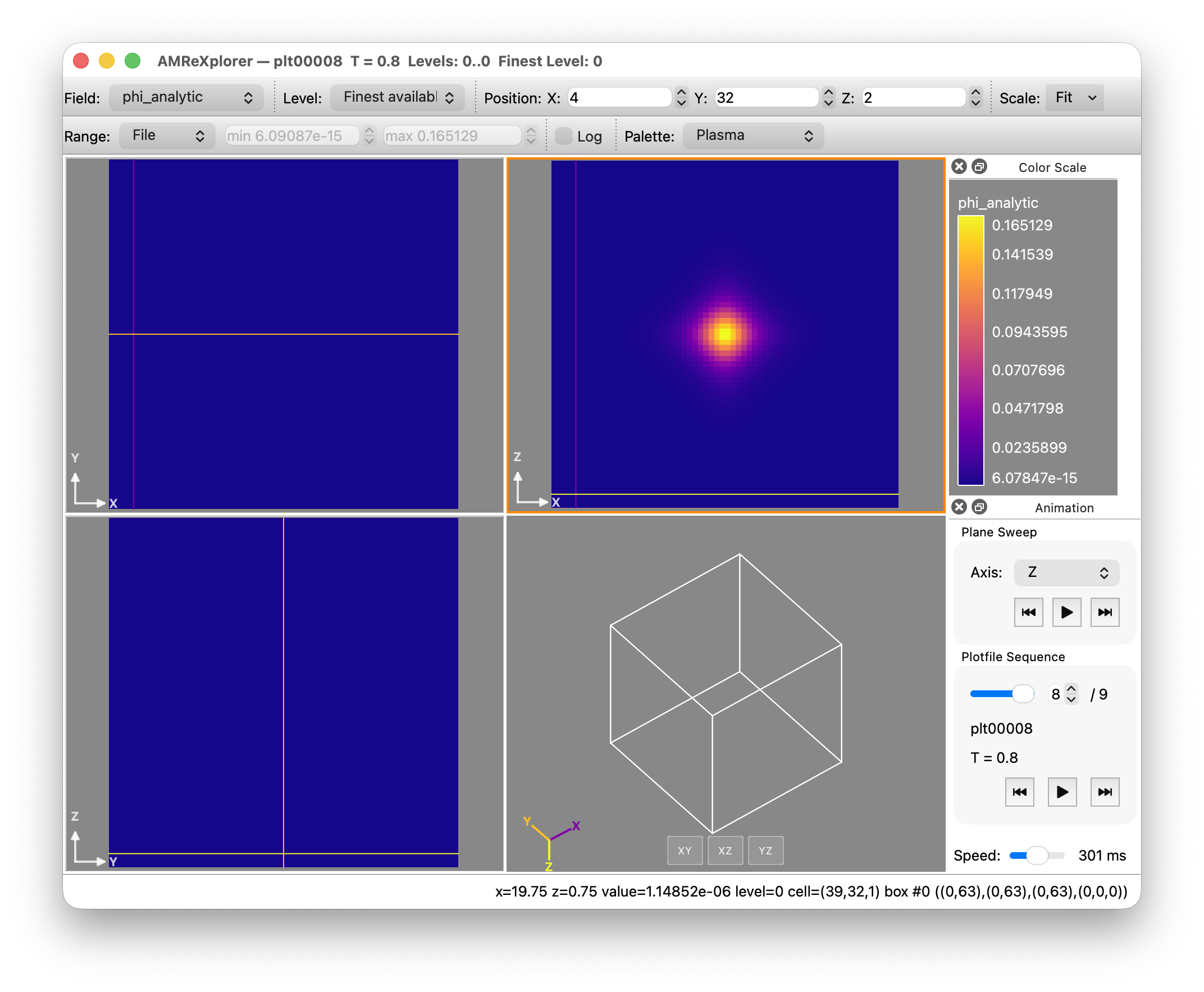
You can then use the "Field" button to scroll through the different variables.
The analytic solution and energy density are examples of GRTeclyn diagnostics (called derived variables by AMReX). See Diagnostics for details of how they are registered, calculated when needed and added to your own example.