Running the scalar field example
Here we explain the scalar field example found in the code, which implements an oscillaton, which is a compact object where the scalar field gradients balance the gravitational attraction, leading to a long-lived, local, oscillating configuration.
The parameters that are provided give a good enough resolution for the physical problem, and can be run relatively quickly on a laptop. For that reason it is a good initial test of running the code. However, to test the performance of the code on a larger system we recommend the Binary BH example.
Physical scenario
This page describes running the Scalar Field example using the parameters found in this parameter file.
Initial data
The initial scalar field profile is set in OscillatonInitialData.hpp.
This uses a quasi-stationary solution obtained from a shooting method, which has then been interpolated using Chebyshev polynomials to give something we can impose analytically. At large radius it reduces to the Schwarzschild metric.
The values for \(\Gamma^i\) could be calculated analytically from derivatives of the conformal metric, but instead we calculate it numerically using the GammaCalculator.hpp tool, which is necessary where the initial data is not conformally flat.
Time-symmetric metric data for the fitted ground-state oscillaton profile is supplied in areal-polar coordinates,
In Cartesian coordinates this is
The CCZ4 variables are chi\(= det(\gamma)^{-1/3} = g_{rr}^{-1/3}\) and h\(= \chi \gamma_{ij}\). The components of the extrinsic curvature K and A\(=\tilde A_{ij}\) are zero. At the initial oscillaton phase the field profile phi is zero and its conjugate momentum Pi is nonzero, which means it can satisfy the constraints for any scalar potential (but it will only be stationary for the massive potential corresponding to the solution).
The conformal connection Gamma\(=\tilde{\Gamma}^i\) is evaluated numerically from h using a separate class GammaCalculator, which is required for consistency since the metric is not conformally flat.
The fitted profiles are finite Chebyshev expansions in
They are smooth and even at the origin.
The geometry approaches a Schwarzschild solution of mass \(M=0.52459888\) at large r.
Note that this profile uses a scalar mass \(\mu=1\) and Newton's constant \(G=1\).
We currently impose a fixed hierarchy of 2:1 refinement grids.
Diagnostics
In this example we show how to extract evolution and diagnostic data along a line through the centre of the oscillaton using the particle interpolator. The field phi is an evolution variable, while the energy density rho is a diagnostic which is calculated only when the extraction requests it. See Diagnostics for more about this distinction.
Further details are below.
Computational set up
Please read the Performance Optimisation guide to understand how to divide the domain into boxes that are shared over the MPI ranks, as this is crucial for obtaining good performance on HPC systems. When GRTeclyn regrids (always at the first step, and at later steps as requested by the user), it will output the grid setup to the output file. This tells you how many boxes are on each level, and what their sizes are. This is very useful for understanding if you are load balancing appropriately.
The parameters should be mostly self explanatory if you are familiar with NR, but you can look at the Parameters guide for more details.
Typically, on an old M1 Macbook laptop with no MPI, we obtain a speed of 650 M/hr in code units with the provided parameters. If your speeds are significantly below this, something is wrong.
Checking the outputs
Viewing 3D data and 2D slices
See Visualising Ouputs for details on visualising. Note that checkpoint files are not viewable with AMReX, only plot files are.
You probably want to look at the scalar profile phi, and perhaps also the conformal factor chi. Both should oscillate during the evolution.
Plots from data files
The example also outputs ASCII data files for post-processing in the extraction_data folder. The files named phi_profile_*.dat contain the scalar field profile and those named rho_profile_*.dat contain the energy density. A separate numbered file is written at each extraction time.
These can be plotted using the Python script plot_lineouts.py found in the example folder. Set its data_path to Path("extraction_data") when running it with the default parameter file.
The resulting image should look like 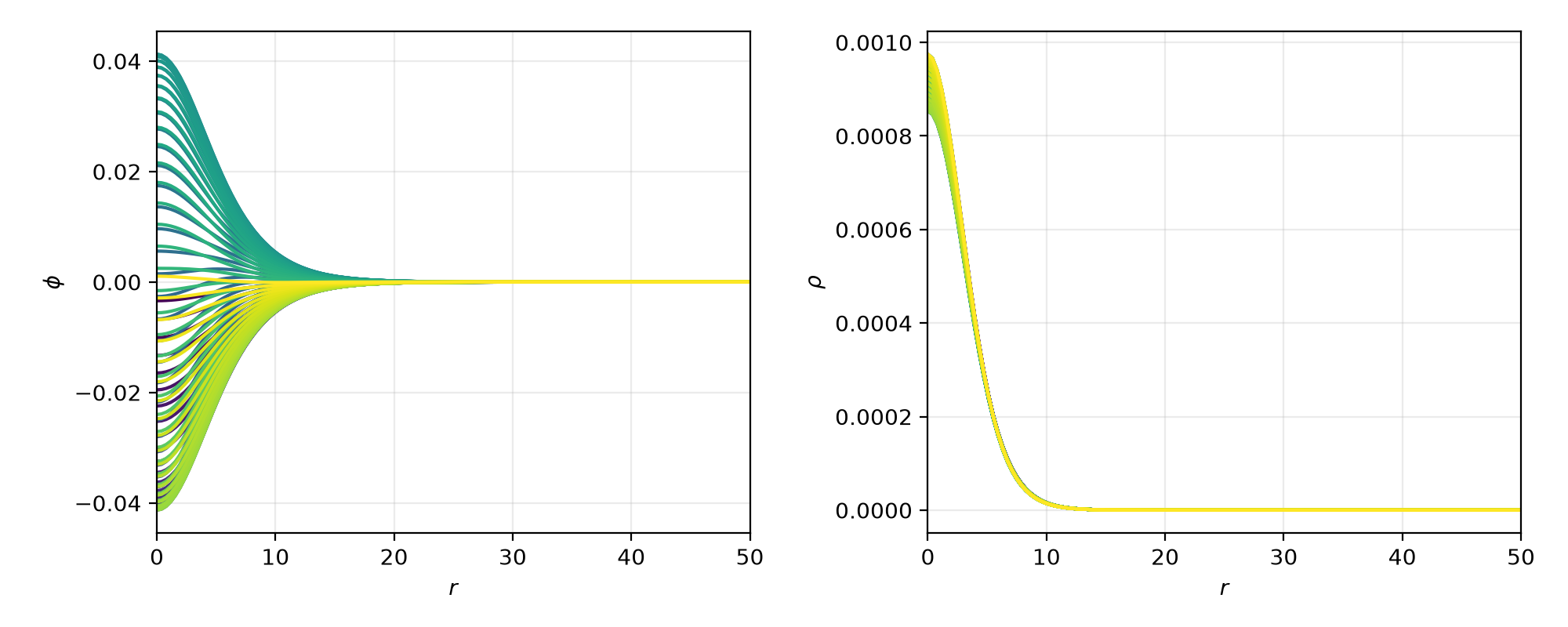
Note that the small oscillation in the density over time is expected - for a real scalar field oscillon, the stress energy tensor is not completely stationary. However, it should not decay noticeably over time and the amplitude of the oscillations should remain just above 0.04.